GradMax¶

GradMax [EMU+22] is a network growing method that focuses on the “how” to grow question, without addressing the “when” and “where” aspects. The objective of this method is to improve the training dynamics of neural networks by finding an interesting way (better than random) to initialize the weights of newly added neurons. To achieve this objective, the gradient of the loss is maximized with respect to the new neurons’ weights, in order to determine how to initialize them.

1. Theory¶

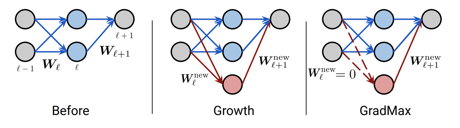
Gradmax: adding a new neuron — Fig. 3 Schematic view of the GradMax algorithm. Growing new neurons requires initializing incoming (\(W_{\ell}^{\text{new}} = \Psi\)) and outgoing (\(W_{\ell+1}^{\text{new}} = \Omega\)) weights for the new neuron. GradMax sets incoming weights to zero (dashed lines) in order to keep the output unchanged, and initializes outgoing weights using SVD. This maximizes the gradients on the incoming weights with the aim of accelerating training. [EMU+22]¶

With \(\Psi = 0\) and \(\sigma(0) = 0\), we have \(a_{-1}^{\text{ext}} = 0\), so \(\nabla_{\Omega} \mathcal{L}(f) = 0\). The loss decrease after one gradient step on \((\Psi, \Omega)\) is:

\[\mathcal{L}(f_{\Psi + \text{d}\Psi}) \approx \mathcal{L}(f) - \|\nabla_{\Psi} \mathcal{L}(f)\|_2^2 - \|\nabla_{\Omega} \mathcal{L}(f)\|_2^2\]

As \(\nabla_{\Psi} \mathcal{L}(f) = 0\) at initialization, GradMax maximizes \(\|\nabla_{\Omega} \mathcal{L}(f)\|_2\).

GradMax solves:

(1)¶\[\Omega^* = \operatorname*{argmax}_{\|\Omega\|_2 \le 1} \|\nabla_{\Psi} \mathcal{L}(f)\|_2\]

such that \(\Omega \Omega^{\top} = I_{C_{\text{ext}}}\).

2. Non-linearities and normalization hypotheses in the case of FC layers¶

Consider fully connected layers with \(\Psi = 0\) and \(\sigma'(0) = 1\):

\[\nabla_{\Psi} \mathcal{L}(f) = \Omega^{\top} \times_C \mathbb{E}_{(x,y) \sim \mathcal{D}} \left[ \nabla_s \mathcal{L}(f)(x) \times_1 a_{-2}(x)^{\top} \right] = \Omega^{\top} \times_C B_{-2}^{\top}\]

The GradMax optimization reduces to:

(2)¶\[\mathcal{J}_{\text{GradMax}}(\Omega) := \|B_{-2} \times_C \Omega\|_2^2\]

such that \(\Omega \Omega^{\top} = I_{C_{\text{ext}}}\).

The optimal \(\Omega^*\) are the leading left-singular vectors of \(B_{-2}\) and scaling them by \(\frac{c}{\|(\sigma_1,\ldots,\sigma_k)\|}\) (where \(\sigma_i\) is the \(i\)-th largest singular value). In order to make a fair comparison between different methods each initialization is scaled such that their norm is equal to the same value, i.e., the mean norm of the existing neurons.

Note

This closed-form solution holds under the hypothesis that the columns of \(\Omega\) are mutually orthonormal, i.e. \(\Omega \Omega^{\top} = I_{C_{\text{ext}}}\). This hypothesis is not explicitly stated in the paper.

3. A few comments¶

Using an iterative method such as projected gradient descent to solve directly (1) (GradMaxOpt) does not work as well as using the SVD, highlighting the benefit of having a closed-form solution. However, if the outgoing weights are set to zero (\(\Omega = 0\)) instead of the incoming weights, then the solution can no longer be found using SVD, and direct optimization of (2) could provide a solution. This could be preferable in some situations since it removes the constraints on the activation function. Moreover, it can avoid the unstable behavior of functions such as batch normalization.
Note that it is feasible to also use the singular values to guide where and when to grow, since the singular values are equal to the value of the maximized optimization problem above. For example, neurons could be added when the singular values meet a certain threshold, and layers to grow could be chosen depending on which have the largest singular values. In their implementation, the authors handle these questions as follows:
- When: neurons are added at fixed intervals during training, independently of the network’s performance. For example every 5 epochs, starting after 20 warmup epochs.
- Where: the retained singular vectors are those associated with the largest singular values. These are the directions along which adding a neuron would maximally increase the gradient norm.
The “Random” baseline used in the experiments sets the incoming weights of each new neuron to zero. Its outgoing weights are sampled from a uniform distribution \(\mathcal{U}([0, 1))\), then each weight vector is divided by its \(\ell_2\)-norm to project it onto the unit sphere. The result is then rescaled by \(0.5 \times\) the mean \(\ell_2\)-norm of the existing neurons, so the new neuron is initialized at half the average magnitude of the neurons already present in the layer. This is not a classical initialization method (e.g., Xavier or Kaiming) since it only set positive weights.

4. Experiments results¶

Baseline-S (small) refers to the seed architecture and Baseline-B (big) to the target architecture. For all architectures, the number of neurons in each layer is reduced by a factor of 4 to obtain the seed architecture.

Table 6 Test accuracy of different baselines and growing methods on different tasks. All results are averaged over 3 random seeds.¶
Dataset	Architecture	Baseline-S	Baseline-B	Random	Firefly	GradMax
CIFAR-10	WRN-28-1	\(89.9 \pm 0.3\)	\(92.9 \pm 0.2\)	\(\mathbf{90.6 \pm 0.2}\)	\(\mathbf{90.8 \pm 0.3}\)	\(\mathbf{91.1 \pm 0.1}\)
CIFAR-10	VGG11	\(84.1 \pm 0.1\)	\(86.6 \pm 0.3\)	\(83.8 \pm 0.6\)	\(84.0 \pm 0.2\)	\(84.4 \pm 0.4\)
CIFAR-100	WRN-28-1	\(63.7 \pm 0.0\)	\(69.3 \pm 0.1\)	\(\mathbf{66.7 \pm 0.4}\)	\(66.5 \pm 0.1\)	\(\mathbf{66.8 \pm 0.2}\)
ImageNet	Mobilenet-V1	\(55.0 \pm 0.0\)	\(70.8 \pm 0.0\)	\(66.9 \pm 0.3\)	\(66.4 \pm 0.1\)	\(\mathbf{68.6 \pm 0.2}\)

Hyperparameters:

Optimizer: SGD with momentum 0.9, weight decay \(2 \times 10^{-4}\), base learning rate \(\eta_0 = 0.1\) for Wide-ResNet an with cosine decay and \(\eta_0 = 0.05\) for VGG

Table 2 shows the effect of using batch normalization or setting outgoing weights to zero, when growing residual networks on CIFAR-10. Batch normalization has limited effect on results. However, setting the outgoing weights to zero yields consistent improvements: in this setting the SVD closed-form solution no longer applies, so GradMaxOpt (iterative optimization of (1)) is used instead, and it outperforms both random initialization and Firefly [WLSL20].

Table 7 Average test accuracy when growing WRN-28 on CIFAR-10 with batch normalization and outgoing weights set to zero. When the outgoing weights are set to zero, GradMaxOpt is used.¶
BN	Inverse	Baseline-S	Baseline-B	Random	Firefly	Gradmax(-Opt)
✗	✗			\(90.6 \pm 0.2\)	\(90.8 \pm 0.3\)	\(91.1 \pm 0.1\)
✗	✓	\(89.9 \pm 0.3\)	\(92.9 \pm 0.2\)	\(92.1 \pm 0.2\)	\(92.2 \pm 0.2\)	\(92.4 \pm 0.1\)
✓	✗			\(92.9 \pm 0.1\)	\(92.9 \pm 0.1\)	\(93.0 \pm 0.1\)
✓	✓	\(90.2 \pm 0.3\)	\(93.4 \pm 0.1\)	\(92.8 \pm 0.1\)	\(92.8 \pm 0.2\)	\(92.9 \pm 0.2\)

Conclusions¶

GradMax is systematically worse than the big baseline.
GradMax outperforms “Random” and “Firefly” in the experiments without batch normalization. However “Random” is a very awkward random initialization method, and in the inverse setting (outgoing weights set to zero) or with batch normalization, GradMax and “Random” perform similarly.
Setting the outgoing weights to zero is a better choice than setting the incoming weights to zero without batch normalization.

Open Questions¶

How does GradMax compare to a more classical random?
How well does the “when” and “where” strategy based on singular values perform?

References¶

[EMU+22] (1,2)

Utku Evci, Bart van Merrienboer, Thomas Unterthiner, Fabian Pedregosa, and Max Vladymyrov. GradMax: Growing Neural Networks using Gradient Information. In ICLR. 2022. URL: https://openreview.net/forum?id=qjN4h_wwUO.

[WLSL20]

Lemeng Wu, Bo Liu, Peter Stone, and Qiang Liu. Firefly Neural Architecture Descent: a General Approach for Growing Neural Networks. In NeurIPS. 2020. URL: https://proceedings.neurips.cc/paper_files/paper/2020/hash/fdbe012e2e11314b96402b32c0df26b7-Abstract.html.