AutoGrow
TLDR: Automatic depth discovery for convolutional networks. Periodically stack new blocks with random (non function-preserving) initialisation and a constant learning rate, and stop growing each sub-network once its growth no longer improves validation accuracy.
AutoGrow [WYCL20] considers the problem of increasing the number of blocks in ResNet [HZRS16] and VGG [SZ15] style architectures, by organising the network into several “stages”. The first block in each stage implements a downsampling of the spatial resolution, after which the spatial resolution is fixed for the remaining blocks in that stage. By increasing the number of blocks, one can grow the network to an arbitrary depth while respecting shape constraints. Starting from the shallowest possible seed (one sub-module per stage), AutoGrow periodically stacks new sub-modules and freezes the depth of a stage as soon as further growth no longer improves validation accuracy. AutoGrow contests the Net2Net notion that function-preserving morphisms are the best way to initialise new layer weights, and instead prefers random initialisation. In addition, AutoGrow shows that growing before convergence leads to better results than waiting for convergence before growing, a finding contested by later layer-growing studies like FRAGrow.
Vocabulary
A network is a cascade of sub-networks, each composed of sub-modules sharing the same output spatial size. A sub-module is the elementary growing unit:
in a ResNet, a sub-module is a residual block;
in a VGG-BN-like plain network, a sub-module is a stack of convolution, Batch Normalization and ReLU.
The notation Basic3ResNet-a-b-c denotes a 3-stage ResNet with
\(a\), \(b\), \(c\) sub-modules per stage;
Basic4ResNet-a-b-c-d is the 4-stage ImageNet variant;
Bottleneck4ResNet uses bottleneck blocks, and PlainMNet the
shortcut-free counterpart.
Examples:
ResNet-20:
Basic3ResNet-3-3-3ResNet-18:
Basic4ResNet-2-2-2-2ResNet-34:
Basic4ResNet-3-4-6-3ResNet-50:
Bottleneck4ResNet-3-4-6-3
Algorithm
AutoGrow maintains a circular list of sub-networks that are still allowed to grow. Every \(K\) epochs the algorithm:
Grows: if the growing policy fires, stacks a new sub-module on top of the current growing sub-network, initialises it, and advances to the next sub-network in the list;
Stops: if the stopping policy fires, permanently removes the most recently grown sub-network from the list.
When the list is empty, AutoGrow fine-tunes the discovered network for \(N_{\text{fine-tune}}\) additional epochs with a standard staircase learning rate schedule.
How
Four sub-module initialisers are studied. In every case, all layers of the new sub-module use default random initialisation, except for the last Batch Normalization layer of the residual sub-module, which receives special treatment:
ZeroInit: the last BN scale is zeroed, making the residual block compute the identity — a function-preserving morphism in the spirit of Net2Net and Network Morphism.AdamInit: every parameter except the last BN of the new sub-module is frozen and the last BN is trained with Adam for at most \(10\) epochs, until the deeper net matches the training accuracy of the shallower one (typically converges in \(<3\) epochs). Treated as an approximate network morphism.UniInit: random uniform initialisation of the last BN with standard deviation \(1.0\) (not function-preserving).GauInit: random Gaussian initialisation of the last BN with standard deviation \(1.0\) (not function-preserving).
The best results use GauInit.
Where
Growth is applied to every sub-network in round-robin order. The seed network has one sub-module per sub-network; depth is grown and stops independently at each resolution stage.
When
Two growing policies are studied:
Periodic Growth (p-AutoGrow): always grow every \(K\) epochs, with a small \(K\) (typically \(K=3\)) so that growth happens before the shallower net converges.
Convergent Growth (c-AutoGrow): grow only once the current network has converged (in practice \(K=200\)).
The stopping policy is the same in both cases: a sub-network stops when validation accuracy improves by less than \(\tau = 0.05\%\) over the last \(J\) epochs. Because p-AutoGrow grows much faster than it converges, \(J\) must be substantially larger than \(K\); the authors recommend \(J=T\), where \(T\) is the number of epochs used at the largest learning rate when training a non-growing baseline (e.g. \(J=100\) on CIFAR, \(J=30\) on ImageNet).
Experimental results
Experiments use SGD with momentum \(0.9\). Baselines use a staircase learning rate (initial \(0.1\) for ResNets, \(0.01\) for plain networks). On CIFAR/SVHN/MNIST, baselines are trained for \(N_{\text{fine-tune}}=200\) epochs with decays at epoch \(100\) and \(150\); on ImageNet, \(N_{\text{fine-tune}}=90\) epochs with decays at \(30\) and \(60\). Except for one ablation study, the experiments use a fixed initial learning rate during growth and use the staircase schedule only for the final fine-tuning. For growing networks, the training time is dependent on the stopping criterion described above.
Non function-preserving initialisation is better
Across both the convergent and periodic regimes, random
initialisation of the last batch normalisation (UniInit,
GauInit) outperforms its function-preserving counterparts
(ZeroInit, AdamInit), with GauInit winning in every
setting. It is important to note that the function-preservation is obtained
through tuning of only the BN scale, which is a very small subset of the parameters of the new
sub-module. It is possible that this conclusion does not hold
for function-preservation obtained by constraining a larger subset of the parameters
(e.g. a full layer).
In the convergent regime (c-AutoGrow with a constant learning
rate), GauInit reaches the best accuracy on both CIFAR-10 and
CIFAR-100:
initialiser |
CIFAR-10 |
CIFAR-100 |
||
|---|---|---|---|---|
found net |
accu (%) |
found net |
accu (%) |
|
|
2-2-4 |
92.23 |
3-2-4 |
70.22 |
|
3-4-4 |
92.60 |
3-3-3 |
70.00 |
|
3-4-4 |
92.93 |
4-4-3 |
70.39 |
|
2-4-3 |
93.12 |
3-4-3 |
70.66 |
In the periodic regime (p-AutoGrow with \(K=3\)) the same
ordering holds, and GauInit additionally grows deeper networks
before the stopping criterion triggers:
initialiser |
CIFAR-10 |
CIFAR-100 |
||
|---|---|---|---|---|
found net |
accu (%) |
found net |
accu (%) |
|
|
31-30-30 |
93.57 |
26-25-25 |
73.45 |
|
37-37-36 |
93.79 |
27-27-27 |
73.92 |
|
28-28-28 |
93.82 |
41-41-41 |
74.31 |
|
42-42-42 |
94.27 |
54-53-53 |
74.72 |
Do not wait for convergence before growing
Holding the initialiser fixed to GauInit, growing before the
shallower network has converged (small \(K\)) discovers
significantly deeper networks and improves the final accuracy. The
table below compares c-AutoGrow (convergent regime, top row) with
p-AutoGrow for several growth periods \(K\):
schedule |
CIFAR-10 |
CIFAR-100 |
||
|---|---|---|---|---|
found net |
accu (%) |
found net |
accu (%) |
|
convergent |
2-4-3 |
93.12 |
3-4-3 |
70.66 |
\(K=50\) |
6-5-3 |
92.95 |
8-5-7 |
72.07 |
\(K=20\) |
7-7-7 |
93.26 |
8-11-10 |
72.93 |
\(K=10\) |
19-19-19 |
93.46 |
18-18-18 |
73.64 |
\(K=5\) |
23-22-22 |
93.98 |
23-23-23 |
73.70 |
\(K=3\) |
42-42-42 |
94.27 |
54-53-53 |
74.72 |
\(K=1\) |
77-76-76 |
94.30 |
68-68-68 |
74.51 |
Accuracy plateaus around \(K=3\): shrinking \(K\) further only adds depth without measurable gain. The trend is studied further in FRAGrow.
The discovered depth is nearly optimal
For a fixed family of architectures, the depth discovered by p-AutoGrow is among the best-performing depths that can be found by training many baselines from scratch.
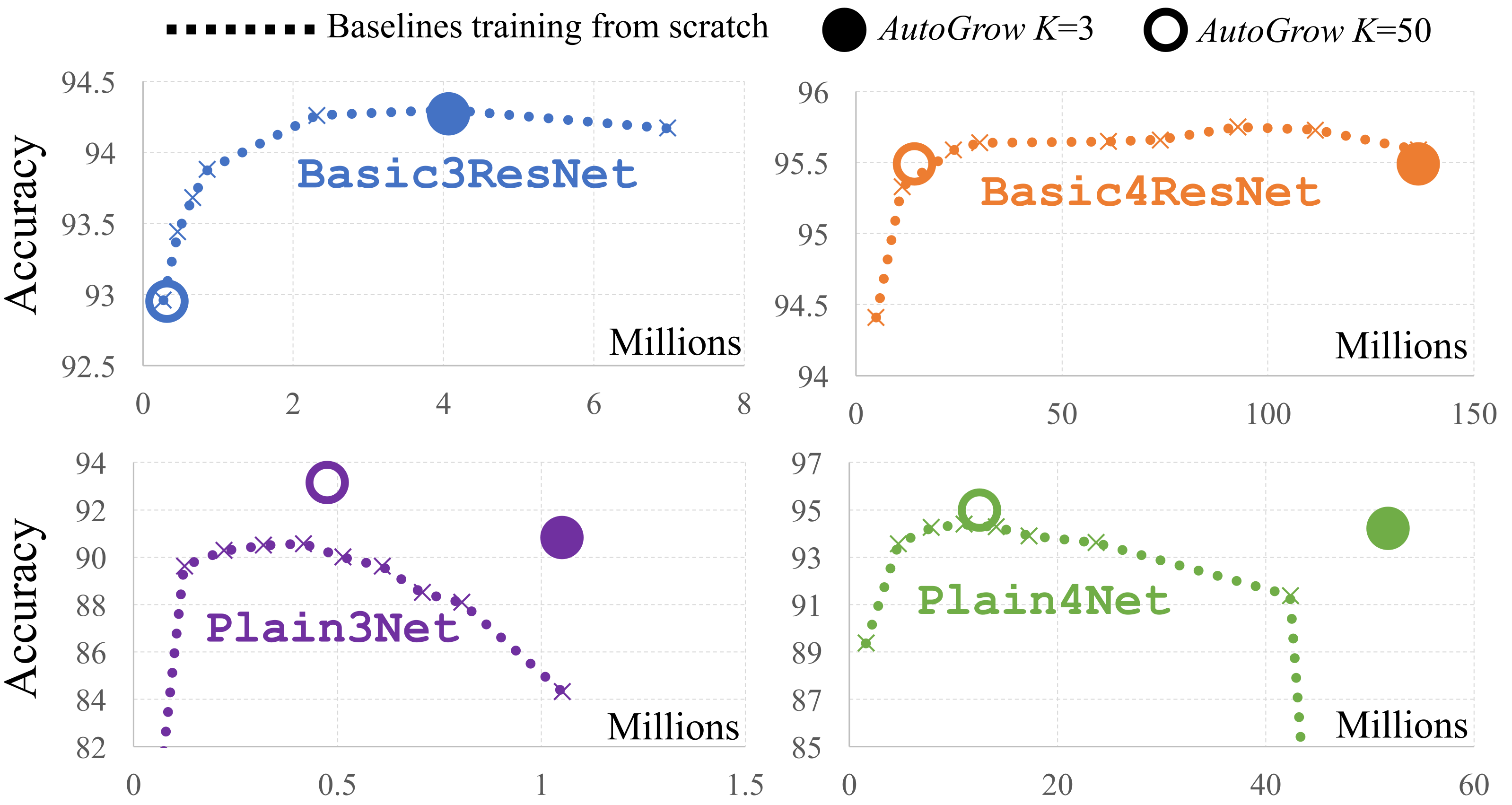
Fig. 3 AutoGrow vs. manual depth search (training many baselines from scratch) on CIFAR-10. Dots \(\bullet\) mark depths discovered by p-AutoGrow with \(K=3\); circles \(\circ\) correspond to \(K=50\). Reproduced from Figure 5 of [WYCL20].
For ResNets the discovered depth lands at the saturation point of the from-scratch curve. For plain VGG-BN networks AutoGrow not only finds a sensible depth but reaches significantly higher accuracy than the from-scratch baseline at the same depth: at those depths the from-scratch baseline fails to train even with batch normalisation, while gradual growth makes deep plain nets trainable. Note that grown networks are trained for more epochs than the from-scratch baselines, which may contribute to the improved accuracy.
AutoGrow only partially adapts to the dataset
Across different datasets, p-AutoGrow (\(K=3\), GauInit)
reaches accuracies close to or above from-scratch training, but the
discovered depth does not obviously reflect dataset complexity —
e.g. CIFAR-100 and CIFAR-10 yield very different depths even though
the inputs are identical, and ImageNet does not yield the deepest
networks despite being the hardest task:
dataset |
found net |
accu (%) |
\(\Delta\) (%) |
|---|---|---|---|
MNIST |
11-10-10-10 |
99.66 |
+0.01 |
FashionMNIST |
27-27-27-26 |
94.62 |
-0.17 |
SVHN |
20-20-19-19 |
97.32 |
-0.08 |
CIFAR-10 |
22-22-22-22 |
95.49 |
-0.10 |
CIFAR-100 |
17-51-16-16 |
79.47 |
+1.22 |
ImageNet |
12-12-11-11 |
76.28 |
+0.43 |
In contrast, when the same dataset is randomly subsampled (with \(K\) rescaled to keep the number of mini-batches between growths constant), the discovered depth shrinks consistently with the dataset size:
Other observations
AutoGrow significantly improves the performance of VGG-BN networks compared to the same architecture trained from scratch. See the plain-network curves in Figure 3: at the depths discovered by AutoGrow, gradual growth bridges the trainability gap that from-scratch training fails to cross.
The depth of the seed network has little impact on the final performance: starting from a deeper seed yields a marginally smaller (and equally accurate) discovered network. The authors recommend the shallowest seed to avoid an extra manual choice.
Connection with other methods. The conclusion that random (non function-preserving) initialisation outperforms function-preserving morphism contradicts Net2Net and Network Morphism.
Limitations
Experiments compare different versions of AutoGrow that lead to different architectures. It is therefore difficult to clearly identify the source of improvement: algorithmic changes that improve the training versus those that improve the architecture.
The inference cost of the produced network is not taken into account.
All experiments are done for only one seed.
References
Kaiming He, Xiangyu Zhang, Shaoqing Ren, and Jian Sun. Deep Residual Learning for Image Recognition. In CVPR. December 2016. arXiv:1512.03385. URL: http://arxiv.org/abs/1512.03385, doi:10.48550/arXiv.1512.03385.
Karen Simonyan and Andrew Zisserman. Very Deep Convolutional Networks for Large-Scale Image Recognition. April 2015. arXiv:1409.1556. URL: http://arxiv.org/abs/1409.1556, doi:10.48550/arXiv.1409.1556.
Wei Wen, Feng Yan, Yiran Chen, and Hai Li. AutoGrow: Automatic Layer Growing in Deep Convolutional Networks. In Proceedings of the 26th ACM SIGKDD International Conference on Knowledge Discovery & Data Mining, KDD '20, 833–841. New York, NY, USA, August 2020. Association for Computing Machinery. URL: https://dl.acm.org/doi/10.1145/3394486.3403126, doi:10.1145/3394486.3403126.